CartPole is a common test for reinforcement learning algorithms with continuous state space.
The Environment.
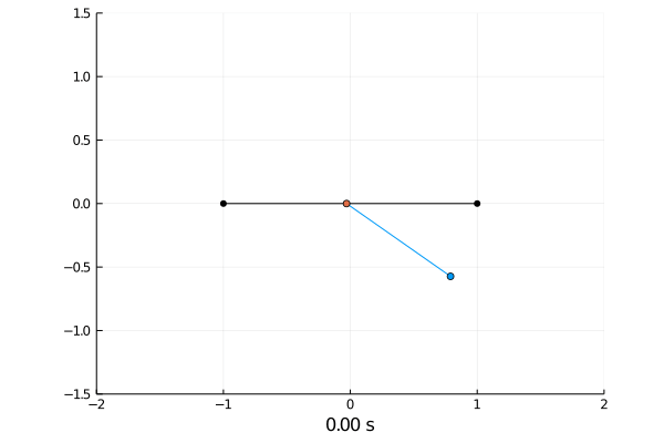
Imagine a cart which can move left and right on a rod. On the center it has a pole attached with a joint so it can move freely in 360 degrees.
The double CartPole has an additional pole attached to the first pole which creates an double pendulum.
The agent has the ability to push the cart left or right with a constant force.
There are packages which already have the CartPole environment implemented but I wanted to do it myself.
The Physics.
Thanks to this blog post I was able to calculate the equations of motion for the cart.
Firstly, we consider a cart with only one pole.
Let \(x \in [x_\min, x_\max]\) denote the horizontal position of the cart and \(v\) its velocity. \(\theta \in [-\pi,\pi]\) is the angle of the pole with respect to the horizontal axis. \(\dot\theta\) is its angular velocity. Lastly, \(m_c\) is the mass of the cart, \(m_p\) is the mass of the pole and \(r\) its length.
To derive the accelerations we take an Lagrangian approach.
The 2d-position of the cart is \begin{align} p_c = \begin{pmatrix} x \\ 0 \end{pmatrix} \end{align} The position of the center of mass of the pole is \begin{align} p_p = p_c + \frac{r}{2} \exp(i\theta) = p_c + \frac{r}{2} \begin{pmatrix} \cos(\theta) \\ \sin(\theta) \end{pmatrix}. \end{align} The cart velocity is \begin{align} v_c = \begin{pmatrix} v \\ 0 \end{pmatrix} = \begin{pmatrix} \dot x \\ 0 \end{pmatrix} \end{align} and the pole velocity is \begin{align} v_p = v_c + \frac{r}{2} i\exp(i\theta)\dot\theta = v_c + \frac{r}{2} \begin{pmatrix} -\sin(\theta)\dot\theta \\ \cos(\theta)\dot\theta \end{pmatrix}. \end{align}
The kinetic energy of the system is \begin{align} T = \frac{1}{2}m_c \norm{v_c}_2^2+ \frac{1}{2}m_p \norm{v_p}_2^2, \end{align} the potential energy is \begin{align} V = m_c g (p_c)_y + m_p g (p_p)_y, \end{align} where \(g\) is gravitation.
If we collect all paramters of the system as symbolic paramters
\begin{align*}
q = \begin{pmatrix}
x \\ \theta
\end{pmatrix} \quad
\dot q = \begin{pmatrix}
\dot x \\ \dot\theta
\end{pmatrix}
\end{align*}
Lagrangian mechanics tells us that for \(L=T-V\)
\begin{align}
\frac{d}{dt}\frac{\partial L}{\partial \dot q} +
\begin{pmatrix}
f \\
0
\end{pmatrix}
= \frac{\partial L}{\partial q},
\end{align}
where \(f\) is the horizontal force applied to the cart.
This system of equations can then be solved analytically, ideally by a computer algebra system.
If we want to model a second pole with angle \(\theta_2\) with respect to the first pole, angular velocity \(\dot \theta_2\), mass \(m_{p2}\) and length \(r_2\) we simply augment \(q\) and \(\dot q\) by \(\theta_2\) and \(\dot \theta_2\) respectively and add the kinetic and potential energy to \(T\) and \(V.\)
The position is given by
\begin{align}
p_{p2} = p_c + r
\begin{pmatrix}
\cos(\theta) \\
\sin(\theta)
\end{pmatrix}
+ \frac{r_2}{2} \begin{pmatrix}
\cos(\theta + \theta_2) \\
\sin(\theta + \theta_2)
\end{pmatrix}
\end{align}
and the velocity by
\begin{align}
v_{p2} = v_c + r
\begin{pmatrix}
-\sin(\theta)\dot\theta \\
\cos(\theta)\dot\theta
\end{pmatrix}
+ \frac{r_2}{2} \begin{pmatrix}
-\sin(\theta + \theta_2)(\dot\theta + \dot\theta_2) \\
\cos(\theta + \theta_2)(\dot\theta + \dot\theta_2)
\end{pmatrix}.
\end{align}
The resulting system of equations is then very hard to solve but a computer can manage it.
Simulating the dynamics was done by solving the differential equations with the semi implicit Euler scheme.

Reinforcement Learning.
As we have an continuous state space \[s = (x,v,\theta,\dot \theta)^T \in [x_\min, x_\max]\times \R \times [-\pi,\pi] \times \R\] we have to approximate the state action value function \[Q(s,a) \approx \hat Q(s,a;\w).\] I opted for a small neural network:
model = Chain(Dense(4+1, 10, sigmoid), Dense(10, 1))
Learning is done by semi gradient descent \begin{align} \delta_t &\gets R_{t+1} + \gamma \hat Q (S_{t+1}, A_{t+1}; \w_T)- \hat Q (S_t, A_t; \w_t) \\ \w_{t+1} &\gets \w_t + \alpha \delta_t \nabla_\w \hat Q(S_t, A_t; \w_t) \end{align}
Task 1: Balancing.
Here the pole starts in an upright position and the agent receives reward \(+1\) as longs as he can balance the pole. The episode ends if the pole falls.


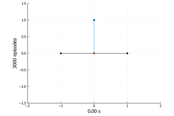

The goal was achieved after 4375 tries.
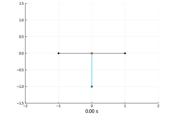
Task 2: Swing up.
Here the pole starts hanging down and the agent has to swing the pole up and then balance it. I have tried several reward signals, like the height of the pole, but the agent did not manage to achieve this task.
So I did a BFS for a solely time dependent swing up policy. With this I was able to swing up the pole in rougly 2 seconds and then balance it with the already trained network (which is time independent).
Double pendulum.
Due to the chaotic behaviour of the double pendulum I did not succeed in training any reasonable agents.