Introduction
The use of machine learning methods in materials science aids human experts in finding task-specific compounds and structures at reduced cost. Specifically, the estimation of materials properties can be accelerated using trained models and applied to large libraries of candidates. However, finding suitable materials descriptors as basis for learning is challenging. Traditional approaches are based on manually crafted features that fulfill all the requirements set by fundamental physics but are best suited for simple fully connected model architectures. Convolutional neural networks based on a three-dimensional grid representation (voxelization), as considered in this work, are a priori much more flexible, but need to be trained not to violate the translation and rotation symmetries of physics.
3D Descriptor
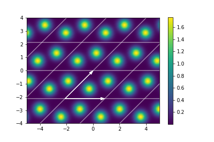
A crystal structure can be thought of as a finite set of atoms repeating along some axes in 3D space. Mathematically, we have a set of Cartesian coordinates \(\bfmu_1, \dots, \bfmu_n \in \R^3\) denoting the positions of \(n\) atoms and a basis \(\bfA := (\bfa_1, \bfa_2, \bfa_3) \in \R^{3\times3}\) along these atoms repeat. If all atom positions are unique and lie in the parallelepiped spanned by the basis \(\bfA\) given by \[\V := \{\bfa_1 x_1 + \bfa_2 x_2 + \bfa_3 x_3: 0 \le x_i \le 1\},\] then \(\V\) is called a unit cell. In this case all atom positions in real space are given by the set \[\{\bfmu_j +\bfA \bfn : \bfn \in \Z^3, j =1,\dots,n\}.\] An example of a 2D crystal structure can be seen in below. The black arrows form the basis.

The key is to describe the crystal structure by some function \(s:\R^3 \to \R\) which satisfies \(s(\bfr + \bfA\bfn) = s(\bfr)\). In this work \(s\) will be a constructed by placing a Gaussian distribution at each atom position, see Figure below.
The periodic function \(s\) can be decomposed in a Fourier series with coefficients indexed by reciprocal vectors, \begin{align*} s(\bfr) &= \sum_{\bfg \in \bfG} h(\bfg)\exp(i\,\bfg\cdot\bfr), \quad \bfr \in \V, \end{align*} where the coefficients are \begin{equation} h(\bfg) = \frac{1}{\operatorname{vol}(\V)}\int_\V s(\bfr) \exp(-i\,\bfg\cdot\bfr)d\bfr. \end{equation}
As already mentioned, for this project the function \(s\) is constructed from Gaussian distributions and is given for \(n\) atoms with Cartesian coordinates \(\bfmu_j\) and basis \(\bfA\) by \begin{align}\label{gaussfield} s(\bfx)&= \sum_{j=1}^n\sum_{\bfn \in\Z^3} \N(\bfx | \bfmu_j + \bfA \bfn, \sigma_j^2 \bfI)\\ &= \sum_{j=1}^n \frac{1}{(2\pi)^{3/2} \sigma_j^3} \sum_{\bfn \in\Z^3}\exp\left(-\frac{1}{2\sigma_j^2}(\bfx - \bfmu_j - \bfA\bfn)^T(\bfx - \bfmu_j -\bfA\bfn)\right). \end{align}
Due to my mathematical background I was able to show that for this special function it holds that \begin{equation}\label{gaussh} h(\bfg) = \frac{1}{|\bfA|} \sum_{j=1}^n \exp\left(-\frac{1}{2}\sigma_j^2 \bfg \cdot \bfg\right) \exp(- i\, \bfg \cdot \bfmu_j). \end{equation} If the standard deviations are chosen to be the same for each atom, \(\sigma_j = \sigma\), above equation simplifies to \begin{equation} h(\bfg) = \frac{1}{|\bfA|} \exp\left(-\frac{1}{2}\sigma^2 \bfg \cdot \bfg\right)\sum_{j=1}^n \exp(- i\, \bfg \cdot \bfmu_j). \end{equation} Computing this expression is much faster than approximating the integral.
Proof.
One Atom at Origin
First, consider the simplest case where we have one atom positioned ate the origin, \(\bfmu = (0,0,0)^T\), \begin{align} s(\bfx) = \sum_{\bfn \in\Z^3} \N(\bfx |\bfA \bfn, \sigma^2 \bfI) \end{align} Recall, that \(\V = \{\bfa_1 x_1 + \bfa_2 x_2 + \bfa_3 x_3: 0 \le x_i \le 1\}\) and \(\operatorname{vol}(\V) = |\bfA|\). Thus by substituting \(\bfA\bfx = \bfr\) we can write the coefficients as \begin{align*} h(\bfg) = \int_0^1\int_0^1\int_0^1 s\left(\bfr\right)\exp(-i\bfg\cdot\bfr)dx_1 dx_2 dx_3, \\ \quad \bfr = x_1\bfa_1+ x_2\bfa_2 + x_3\bfa_3 = \bfA \bfx. \end{align*} Since \(\bfg = \bfB\bfm\) for some \(\bfm \in \Z^3\) and \(\bfB = 2\pi (\bfA^{-1})^T\) we have that \[\bfg \cdot \bfr = (\bfB\bfm)^T(\bfA\bfx) = \bfm^T \bfB^T \bfA \bfx = 2\pi \bfm \cdot \bfx \] and \begin{align*} h(\bfg) &= \int_0^1\int_0^1\int_0^1 s\left(\bfA\bfx\right)\exp(-2\pi i \,\bfm \cdot \bfx)dx_1 dx_2 dx_3 \\ &= \int_0^1\int_0^1\int_0^1 \frac{1}{(2\pi)^{3/2}\sigma^3} \sum_{\bfn \in\Z^3}\exp\left(-\frac{1}{2\sigma^2}(\bfA\bfx - \bfA\bfn)^T(\bfA\bfx - \bfA\bfn)\right)\exp(-2\pi i\, \bfm \cdot \bfx)d\bfx \\ &= \sum_{\bfn \in\Z^3} \int_0^1\int_0^1\int_0^1 \frac{1}{(2\pi)^{3/2}\sigma^3} \exp\left(-\frac{1}{2\sigma^2}(\bfx - \bfn)^T\bfA^T\bfA(\bfx - \bfn)\right)\exp(-2\pi i\, \bfm \cdot \bfx)d\bfx\\ &= \sum_{\bfn \in\Z^3} \int_{-n_3}^{1-n_3}\int_{-n_2}^{1-n_2}\int_{-n_1}^{1-n_1} \frac{1}{(2\pi)^{3/2}\sigma^3} \exp\left(-\frac{1}{2\sigma^2}\bfx^T\bfA^T\bfA\bfx\right)\exp(-2\pi i\, \bfm \cdot \bfx -2\pi i\, \underbrace{\bfm \cdot\bfn}_{\in \Z})d\bfx\\ &= \int_{\R^3}\frac{1}{(2\pi)^{3/2}\sigma^3} \exp\left(-\frac{1}{2\sigma^2}\bfx^T\bfA^T\bfA\bfx\right)\exp(2\pi i\, \bfm \cdot \bfx)d\bfx\\ &= \frac{1}{(2\pi)^3}\int_{\R^3}\frac{1}{(2\pi)^{3/2}\sigma^3} \exp\left(-\frac{1}{2(2\pi\sigma )^2}\bfx^T\bfA^T\bfA\bfx\right)\exp(i\, \bfm \cdot \bfx)d\bfx\\ &= |(\bfA^T\bfA)^{-1}|^{1/2}\int_{\R^3}\frac{1}{(2\pi)^{3/2}|(2\pi\sigma)^2(\bfA^T\bfA)^{-1}|^{1/2}} \exp\left(-\frac{1}{2(2\pi\sigma )^2}\bfx^T\bfA^T\bfA\bfx\right)\exp(i \,\bfm \cdot \bfx)d\bfx\\ &= \frac{1}{|\bfA^T\bfA|^{1/2}}\int_{\R^3} \N(\bfx | \boldsymbol{0}, (2\pi\sigma)^2 (\bfA^T\bfA)^{-1}) \exp(i \,\bfm \cdot \bfx) d\bfx \\ &= \frac{1}{|\bfA|}\exp\left(-\frac{1}{2}(2\pi\sigma)^2 \bfm^T (\bfA^T\bfA)^{-1} \bfm\right) \end{align*} where the last equality follows by substituting the known characteristic function of a Gaussian distribution for the integral. Since \[\bfA^T \bfA \bfB^T \bfB = \bfA^T \bfA 2\pi \bfA^{-1} 2\pi (\bfA^{-1})^T = (2\pi)^2 \bfI\] it holds that \[(2\pi\sigma)^2 \bfm^T (\bfA^T\bfA)^{-1} \bfm = \sigma^2 \bfm^T\bfB^T \bfB \bfm = \sigma^2 \bfg \cdot \bfg \] and the proof is complete.
One Atom at Arbitrary Position
If the atom is placed at position \(\bfmu\), then write \(\bfmu = \bfA\bfnu\) and we have \begin{align*} h(\bfg) &= \int_0^1\int_0^1\int_0^1 s\left(\bfA\bfx - \bfmu\right)\exp(-2\pi i \,\bfm \cdot \bfx)dx_1 dx_2 dx_3 \\ &=\int_{-\nu_3}^{1-\nu_3}\int_{-\nu_2}^{1-\nu_2}\int_{-\nu_1}^{1-\nu_1} s\left(\bfA\bfx\right)\exp(-2\pi i \,\bfm \cdot (\bfx + \bfnu))dx_1 dx_2 dx_3 \\ &= \frac{1}{|\bfA|}\exp(-2\pi i \,\bfm \cdot \bfA^{-1}\bfmu)\exp\left(-\frac{1}{2}(2\pi\sigma)^2 \bfm^T (\bfA^T\bfA)^{-1} \bfm\right) \\ &= \frac{1}{|\bfA|}\exp(- i \,\bfm^T\bfB^T\bfmu)\exp\left(-\frac{1}{2}\sigma^2 \bfm^T\bfB^T\bfB\bfm\right) \\ &= \frac{1}{|\bfA|}\exp(- i \,\bfg \cdot \bfmu)\exp\left(-\frac{1}{2}\sigma^2 \bfg \cdot \bfg\right) \end{align*} The second equality follows by pulling \(\exp(-2\pi i \,\bfm \cdot \bfnu))\) out of the integral and computing the remaining integral as in the previous case.
Multiple Atoms at Arbitrary Positions
For multiple atoms at positions \(\bfmu_i\) all repeat according to \(\bfA\), the equation follows from the previous case due to the linearity of the integral.
\(\Box\)
Relation to Dirac distributions
Note that if \(\sigma=0\), then \begin{align*} h(\bfg) = \frac{1}{|\bfA|} \sum_{j=1}^n \exp(- i \bfg \cdot \bfmu_j), \end{align*} which corresponds to a field quantity consisting of Dirac distributions \begin{align*} s(\bfx) = \sum_{j=1}^n\sum_{\bfn \in\Z^3} \delta_{\bfmu_j + \bfA \bfn}(\bfx). \end{align*}
Properties
Translational invariance. For the translation \(\tilde\bfmu_j := \bfmu_j + \mathbf{t}\), then still \(\tilde\bfA = \bfA\) and \[|\tilde h(\bfg)| = \left|\frac{1}{\operatorname{vol}(\V)}\int_\V s(\bfr - \mathbf{t}) \exp(-i\,\bfg\cdot\bfr)d\bfr\right| = |\exp(-i\, \bfg \cdot \mathbf{t})||h(\bfg)| = |h(\bfg)|.\]
Invariance w.r.t. the choice of unit cell. If \(\bfA\) and \(\tilde\bfA\) are both a basis of a unit cell such that \(\bfmu_j\) repeat according to them, then \(\tilde h(\bfg) = h(\bfg)\) since \(|\tilde\bfA| = \operatorname{vol}(\V) = |\bfA|.\)
Orthogonal transformation equivariance. For an orthogonal matrix \(\mathbf{Q}\), we can make the coordinate change \(\tilde \bfA := \mathbf{Q} \bfA\), \(\tilde\bfmu_j := \mathbf{Q} \bfmu_j\) and obtain \[\tilde \bfB = 2\pi (\tilde\bfA^{-1})^T = 2\pi (\bfA^{-1}\mathbf{Q}^T)^T = 2\pi \mathbf{Q}(\bfA^{-1})^T = \mathbf{Q} \bfB\] such that for \(\tilde \bfg := \tilde\bfB\bfm\) and \(\bfg := \bfB\bfm\) we have \begin{align*} \tilde h(\tilde \bfg) & = \frac{1}{|\tilde\bfA|} \sum_{j=1}^n \exp\left(-\frac{1}{2}\sigma_j^2 \tilde\bfg \cdot \tilde\bfg\right) \exp(- i \,\tilde\bfg \cdot \tilde\bfmu_j) \\ &= \frac{1}{|\tilde\bfA|} \sum_{j=1}^n \exp\left(-\frac{1}{2}\sigma_j^2 \tilde\bfB\bfm \cdot \tilde\bfB\bfm\right) \exp(- i\, \tilde\bfB\bfm \cdot \tilde\bfmu_j) \\ &= \frac{1}{|\mathbf{Q}\bfA|} \sum_{j=1}^n \exp\left(-\frac{1}{2}\sigma_j^2 \bfm^T\bfB^T \mathbf{Q}^T \mathbf{Q}\bfB\bfm\right) \exp(- i \,\bfm^T \bfB^T\mathbf{Q}^T \mathbf{Q}\bfmu_j) \\ & = \frac{1}{|\bfA|} \sum_{j=1}^n \exp\left(-\frac{1}{2}\sigma_j^2 \bfm^T\bfB^T \bfB\bfm\right) \exp(- i \,\bfm^T \bfB^T\bfmu_j) = h(\bfg). \end{align*} Therefore, for rotations, reflections, and rotoreflections of the real space, the reciprocal space undergoes the same transformation.
Having calculated the coefficients it remains to discretize them to a 3D array. In order to do so, a grid is centered at the origin of the reciprocal space and the absolute values \(|h(\bfg)|\) are placed according to their position \(\bfg\). This process is illustrated in Figure below. In this project I considered the same descriptor as in Kajita et al. (2017) and also tried a descriptor in spherical coordinates. The number of grid points along one axis is given by parameter \(N\) and the size of the grid is controlled by parameter \(L\) such that the width for the Cartesian descriptor is \(2 \pi N / L\) and the diameter for the spherical descriptor is \(2 \pi N / L \cdot \sqrt{d}\), where \(d\) is the number of dimensions. Taking rotations into account both descriptors can describe the same information for same parameters (\(2 \pi N / L \cdot \sqrt{d}\) is also the length of the diagonal of the square).


Figure: Top: Reciprocal space with coefficients. Left: Cartesian descriptor. Right: Spherical descriptor.
Training a CNN
For this project two data sets were collected by querying the openly available AFLOW database through the third party Python API aflow. The AFLOW database contains multiple entries for the same compound. For simplicity, duplicates were dropped and only the first fetched entries were used. From the attributes \(\texttt{geometry}\) and \(\texttt{positions_fractional}\) the unit cell basis \(\bfA\) and the Cartesian coordinates of each atom \(\bfmu_j\) are calculated. The target variable is chosen to be enthalpy per atom given by the attribute \(\texttt{enthalpy_atom}\). The enthalpy of a system is defined as the sum of its internal energy and the product of its pressure and volume, i.e., \(H = E + PV\). After filtering out compounds with infrequent elements a total of 5237 compounds comprised of 72 distinct elements remain.
The convolutional neural network architecture from Kajita et al. was adapted and implemented in PyTorch. It will be referred to as VoxelNet. An overview of its architecture and intermediate tensor shapes can be seen below.

Due to poor performance the batch normalization layer which follows the first convolutional layer in the CNN was dropped in favor of SELU activation functions. The VoxelNet has approximately 80000 parameters depending on the number of elements.
For training purposes, a custom class following Python's generator pattern was implemented in order to have fine control over the data augmentation. Kajita et al. augmented the data by rotating each compound 30 times to a larger fixed data set. However, for this project each compound was randomly rotated and reflected each time it is fed into the CNN. Also rather than applying the transformations directly to the \(M\times N \times N \times N\) tensors, they were applied to the reciprocal vectors and the discretization is computed on the fly. This avoids interpolation that would be required in a tensor rotation and it is more RAM efficient as only the descriptors for the current batch have to be stored. The batch-size $B$ was fixed at 64 and the ADAM optimizer with learning rate \(0.001\) and regularisation parameter \(\lambda\) was employed. The descriptor size was set to \(N=32\). The data sets were split into a training (80%), validation (10%) and test (10%) set. After 50 epochs the neural network weights performing best on the validation set were evaluated on the test set.
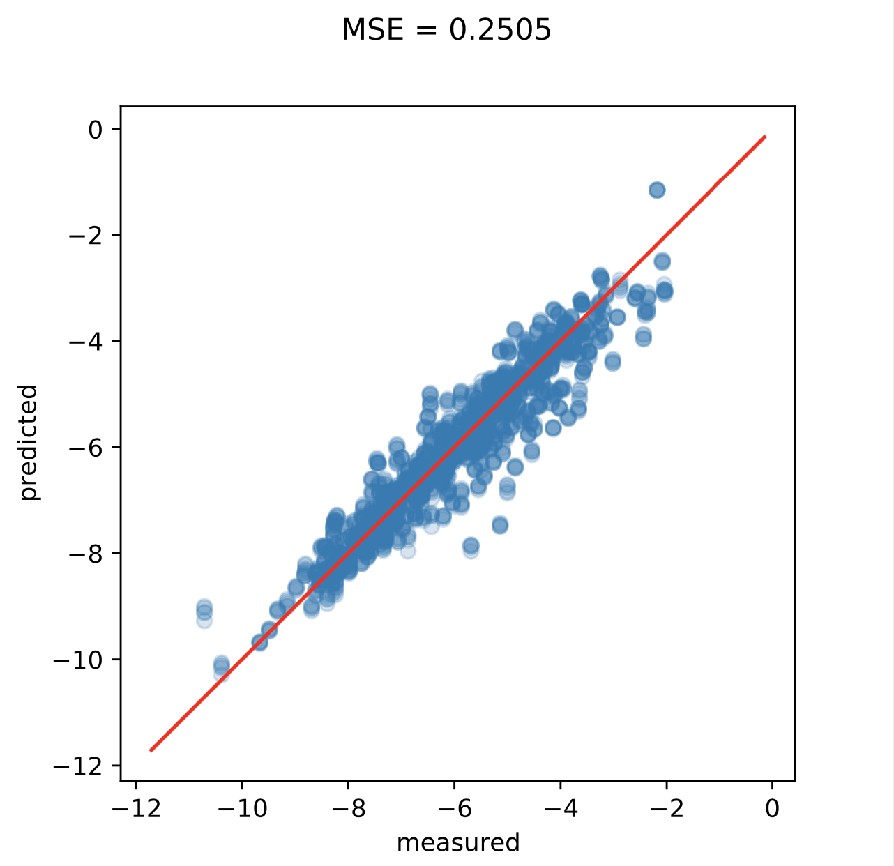
Below you can see the results with hyperparameters \(\sigma = 0.1, L = 12.8,\) and \(\lambda = 0.001.\) compared to some baselines. The prediction accuracy of the VoxelNet was measured first on the original descriptors and a second time where the descriptors for each compound were randomly transformed five times.
| train | test | |
|---|---|---|
| ZeroR | 2.4728 | 2.3399 |
| RidgeR | 0.5674 | 0.6069 |
| MLP | 0.1455 | 0.4117 |
| VoxelNet Cartesian | 0.2486/0.2168 | 0.2986/0.2758 |
| VoxelNet Spherical | 0.2165/0.2000 | 0.2655/0.2505 |
Lastly, below are the plots of accuracy during training and predictions on the augmented test set for the spherical descriptor.