Kulback-Leibler Divergence and Variational Inference

Kulback-Leibler Divergence

The KL-Divergence between two distributions \(P\) and \(Q\) is given by \[\KL(P \parallel Q) = \Exp{X \sim P}{\log\left(\frac{P(X)}{Q(X)}\right)}.\] It is the expected log likelihood ratio. By the Neyman–Pearson lemma this ratio is the most powerful way to distinguish between the two distributions.

The KL-Divergence can be split up into a cross-entropy and entropy term \begin{align} \KL(P \parallel Q) &= \Exp{X \sim P}{-\log Q(X) } - \Exp{X \sim P}{-\log P(X) } \\ &= H(P,Q) - H(P) \end{align}

The KL-Divergence is only well defined if \(Q \ll P\), i.e. \(P(A) = 0 \implies Q(A) = 0.\) Otherwise we can set it to \(\infty.\) Note that \(\KL(P \parallel Q)\) can be infinite even if \(Q \ll P.\)

It holds that \[\KL(P \parallel Q) \ge 0 \quad \text{and} \quad \KL(P \parallel Q) = 0 \iff P = Q. \]

The KL-Divergence is asymmetric, because \(P\) determines over which support the log likelihood ratio is averaged. For example, if we want to approximate a bimodal Gaussian mixture model \[P(x) = 0.4 \cdot \N(x \mid {-1}, 0.75^2) + 0.6 \cdot \N(x \mid 4, 0.5^2), \] with an unimodel Gaussian \[Q(x) = \N(x \mid \mu, \sigma^2),\] then it matters whether we minimize \(\KL(P \parallel Q)\) or \(\KL(Q \parallel P).\)

The first case is called the inclusive KL, where \(Q\) will try to minimize the distance of the densities on the support of \(P\) (see left plot below), while in the second case, the exclusive KL, \(Q\) will match the Normal distribution with the higher probability (see right plot below).

Variational Inference

Lets suppose our data comes from a bimodal Gaussian mixture model \[P(x \mid \bfmu) = 0.5 \cdot \N(x \mid \mu_1, 0.5) + 0.5 \cdot \N(x \mid \mu_2, 0.5), \] and we have observed \[\D = [ 1.41, -1.07, -0.85, -1.05, -0.21, 0.62, -0.59, -1.09, -0.24, 1.11].\] We would like to infer the correct centers \(\bfmu.\)

In the usual Bayesian fashion, we want to find the posterior \[\Prob{\bfmu \mid \D} = \frac{\Prob{\D \mid \bfmu} \Prob{\bfmu} }{\Prob{\D} }.\]

We choose an uniform prior \(\Prob{\bfmu} = \text{Unif}(\bfmu \mid [-2,2] \times [-3,3])\) and use MCMC to sample from the posterior (see 1 and 2). We visualise the samples with the 2D kernel density:

To find the two modes we had to sample over a million times. Another method to approximate the posterior is variational inference.

In variational inference we aim to approximate the posterior with a simpler distribution over the latent variables \(q_\theta(z),\) and minimize the KL-divergence with respect to the parameters \(\theta\) \[\KL(q_\theta, \Prob{.\mid \D)}.\] In our case \(z = \bfmu.\)

But how to measure this distance if we do not have access to the posterior \(\Prob{.\mid \D}?\) Well, we are Bayesians, so we use the fact that \[\Prob{z \mid \D} = \frac{\Prob{\D \mid z}\Prob{z}}{\Prob{\D}} = \frac{\Prob{\D , z}}{\Prob{\D}}\] and substitute in the definition of the KL-divergence \begin{align} \KL(q_\theta \parallel \Prob{.\mid \D)} &= \Exp{Z \sim q_\theta}{\log\left(\frac{q_\theta(Z)}{\Prob{Z \mid \D}}\right) } \\ &= \Exp{Z \sim q_\theta}{\log\left(\frac{q_\theta(Z) \Prob{\D}}{\Prob{\D , z}}\right) } \\ &= \Exp{Z \sim q_\theta}{\log\left(\frac{q_\theta(Z) }{\Prob{\D , z}}\right) } + \Exp{Z \sim q_\theta}{\log\Prob{\D} } \\ &= \KL(q_\theta \parallel \Prob{., \D}) + \log\Prob{\D} \\ &= -\text{ELBO}(q_\theta) + \log\Prob{\D} \end{align}

Since \(\log\Prob{\D}\) is constant we can minimize \(\KL(q_\theta \parallel \Prob{.\mid \D)}\) by maximizing the so-called evidence-lower-bound, which is tractable.

Indeed, \(\text{ELBO}(q_\theta)\) is a lower bound on the evidence \(\log\Prob{\D},\) \begin{align} \underbrace{\log\Prob{\D}}_{\le 0} = \underbrace{\KL(q_\theta \parallel \Prob{.\mid \D)}}_{\ge 0} + \underbrace{\text{ELBO}(q_\theta)}_{\le 0} \ge \text{ELBO}(q_\theta). \end{align}

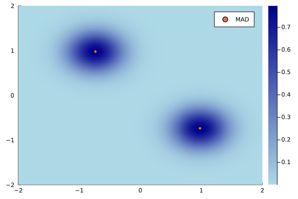
For our model \[P(x \mid \bfmu) = 0.5 \cdot \N(x \mid \mu_1, 0.5) + 0.5 \cdot \N(x \mid \mu_2, 0.5), \] we can make an informed guess about how the posterior could be efficiently approximated. First note that \(\mu_1\) and \(\mu_2\) can be interchanged which we reflect in \(q_\bfmu,\) \[q_{(\mu_1, \mu_2)}(z) = q_{(\mu_2, \mu_1)}(z). \] Also because of this fact there should be two equivalent modes. They should become Guassian with increased number of observations. Therefore, we select \[q_{\bfmu}(z) = 0.5 \cdot \N(z \mid \mu_1, \sigma^2) + 0.5 \cdot \N(z \mid \mu_2, \sigma^2), \] with a fixed standard deviation \(\sigma = 0.1.\)

Maximizing the \(\text{ELBO}\) gives us \(\bfmu = (0.98, -0.74)\) which is close to the true parameter \((1.0,-1.0).\) Below you can see the density of \(q_{\bfmu}\) with the two mirrored modes.

Relation to Maximum Likelihood Estimation

The minimizer of the KL-divergence is the MLE with infinite observations and true parameter \(\theta^*\) in the following sense. \begin{align} \theta_\text{MLE} &= \text{arg max}_\theta \enspace q_\theta(\D) = \text{arg max}_\theta \sum_{i=1}^N \log q_\theta(x_i) \\ &= \text{arg max}_\theta \sum_{i=1}^N \log q_\theta(x_i) - \log q_{\theta^*}(x_i) \\ &= \text{arg max}_\theta \frac{1}{N} \sum_{i=1}^N \log\left(\frac{q_\theta(x_i)}{q_{\theta^*}(x_i)}\right)\\ &\to \text{arg max}_\theta \enspace \Exp{X \sim q_{\theta^*}}{\log\left(\frac{q_\theta(X)}{q_{\theta^*}(X)}\right)} \\ &= \text{arg min}_\theta \enspace \KL(q_\theta \parallel q_{\theta^*}) \end{align}

where \(\D = (x_1, \dots x_N) \sim p_{\theta^*}\) iid.

Furthermore, note that with uniform priors the MAP coincides with the MLE, \begin{align} \text{arg max}_z \enspace \Prob{z \mid \D} = \text{arg max}_z \frac{\Prob{\D \mid z}\Prob{z}}{\Prob{\D}} = \text{arg max}_z \enspace \Prob{\D \mid z}. \end{align}

For optimization source code see my github.