Z - tests
Test for Normal Mean - Known Variance
For \(X = X_1, \dots, X_n \sim \N(\mu,\sigma^2)\), iid. \[\Null: \mu = \mu_0\] \[\frac{\overline X - \mu_0}{\sigma / \sqrt{n}} \sim \N(0,1)\]
Test for Proportion / Binomial test
If \(X = X_1, \dots, X_n \sim \text{Bernoulli}(p)\) then \[\overline X \sim \frac{1}{n}\text{Binom}(n,p) \approx \N(p, p(1-p)/n)\] and \[\Null: p = p_0\] \[\frac{\overline X - p_0}{\sqrt{p_0(1-p_0) / n}} = \frac{k - n p_0}{\sqrt{np_0(1-p_0)}} \approx \N(0,1)\] where \(k = \sum_{i=1}^n X_i \sim \text{Binom}(n,p).\)
Test for Difference in Proportion
If there are is a second sample \(Y = Y_1, \dots, Y_m \sim \text{Bernoulli}(q)\) we can test for difference in proportions. \[\Null: p - q = w_0\] \[\frac{\hat p - \hat q - w_0}{\hat \sigma} \approx \N(0,1)\] with \(\hat p = \overline X,\) \(\hat q = \overline Y,\) \[\bar p = \frac{n \hat p + m \hat q}{n+m}, \quad \hat\sigma = \sqrt{\bar p(1-\bar p)\left(\frac{1}{n}+ \frac{1}{m}\right)}.\]
In all proportion tests we should have more than 30 samples.
Student's t tests
One sample
For \(X = X_1, \dots, X_n \sim \N(\mu,\sigma^2)\), iid. \[\Null: \mu = \mu_0\] \[\frac{\overline{X} - \mu_0}{S_X / \sqrt{n}} \sim t_{n-1}\]
Note that here we have "equality". In the proportion test we only have an approximation. We have \(t_n \to \N(0,1)\) and for \(n > 30\) the approximation is good enough.
Two independent samples (unpaired)
Common variance. For \(X = X_1, \dots, X_n \sim \N(\mu_X,\sigma^2)\), iid., \(Y = Y_1, \dots, Y_m \sim \N(\mu_Y,\sigma^2)\), iid. \[\Null: \mu_X - \mu_Y = w_0\] \[ \frac{\overline X - \overline Y - w_0}{S_p \sqrt{\frac{1}{n} + \frac{1}{m}}} \sim t_{n+m-2} \] where \[S_p = \sqrt{\frac{(n-1)S_X^2 + (m-2)S_Y^2}{n+m-2}}\] is the pooled standard deviation. \(S_p^2\) is an unbiased estimated for \(\sigma^2\).
Can be applied if \(0.5 < S_X / S_Y < 2\).
If \(m=n\) \[ \frac{\overline X - \overline Y - w_0}{S_p \sqrt{\frac{2}{n}}} \sim t_{2n-2}, \] \[S_p = \sqrt{\frac{S_X^2 + S_Y^2}{2}}.\]
Unequal variance - Welch test. For \(X = X_1, \dots, X_n \sim \N(\mu_X,\sigma_X^2)\), iid., \(Y = Y_1, \dots, Y_m \sim \N(\mu_Y,\sigma_Y^2)\), iid. \[\Null: \mu_X - \mu_Y = w_0\] \[ \frac{\overline X - \overline Y - w_0}{\overline S} \approx t_\nu, \quad \text{where} \quad \overline S = \sqrt{\frac{S_X^2}{n} + \frac{S_Y^2}{m}}, \] \[ \nu = \left(\frac{S_X^2}{n} + \frac{S_Y^2}{m}\right)^2 {\huge/} \left(\frac{(S_X^2/n)^2}{n-1} + \frac{(S_Y^2/m)^2}{m-1} \right) \] Recommended: \(m \approx n\), \(m,n > 30\).
Two dependent samples (paired)
For \(X = X_1, \dots, X_n\), iid., \(Y = Y_1, \dots, Y_n \), iid. Requirement: Differences \(D_i = X_i - Y_i\) are independent and (approximately) \(\overline D \sim \N(\mu_D,S_D^2/n).\) \[\Null: \mu_X - \mu_Y = w_0\] \[\frac{\overline{D} - w_0}{S_D / \sqrt{n}} \sim t_{n-1}.\]
F-Tests
Equality of Variance
For \(X = X_1, \dots, X_n \sim \N(\mu,\sigma_X^2)\), iid., \(Y = Y_1, \dots, Y_m \sim \N(\mu,\sigma_Y^2)\), iid. \[\Null: \sigma_X = \sigma_Y\] \[\frac{S_X^2}{S_Y^2} \sim F_{n-1, m-1}\]
one-way ANOVA
Investigation of influence of one factor on random variable by considering the means. It is the generalisation of the two sample t test. \[\Null: \mu_1 = \mu_2 = \dots = \mu_k\]
Requirement: Factor levels have to be independent. Resiuduals must be zero-mean normal with same variance (also between groups).
It is assumed that the observations belonging to a group are the same (-noise) and that the variance is explained by the factor alone. \[y_{ij} = \mu_i + \epsilon_{ij} = \mu + \tau_i + \epsilon_{ij}, \quad i=1,\dots,k, \enspace j=1,\dots,n_i\] where \(\epsilon_{ij} \sim \N(0,\sigma^2)\) iid., \(\mu_i = \mu + \tau_i\) is the influence of the factor and \(n_1+\cdots+n_k=N.\)
We want to find point estimates of \(\mu, \mu_i\) and \(\tau_i\). Let \[\overline y_i = \frac{1}{n_i}\sum_{j=1}^{n_i} y_{ij}, \quad s_i^2 = \frac{1}{n_i-1}\sum_{j=1}^{n_i}(y_{ij}-\overline y_i)^2\] Then the sample man is \[\overline y = \frac{1}{N}\sum_{i=1}^k n_i \overline y_i.\] We take \(\hat \mu = \overline y\), \(\hat \mu_i = \overline y_i\) and \(\hat \tau_i = \hat \mu_i - \hat \mu.\) The residuals are \(\hat \epsilon_{ij} = y_{ij} - \overline y_i.\)
The decomposition of variance is given by \begin{align} \underbrace{\sum_{n=1}^N (y_{n} - \overline y)^2}_{\text{TSS}} = \underbrace{\sum_{n=1}^N (\hat y_{n} - \overline y)^2}_\text{RegSS} + \underbrace{\sum_{n=1}^N (y_n - \overline y)^2}_\text{RSS} \end{align} In our case \(\hat y_{ij} = \overline y_i\) and so \begin{align} \text{TSS} &= \sum_{i=1}^k\sum_{j=1}^{n_i} (y_{ij} - \overline y)^2 \\ \text{RegSS} &= \sum_{i=1}^k n_i (\overline y_i - \overline y)^2 = \sum_{i=1}^k n_i \hat \tau_i^2 \\ \text{RSS} &= \sum_{i=1}^k \sum_{j=1}^{n_i} \hat \epsilon_{ij}^2 = \sum_{i=1}^k\sum_{j=1}^{n_i} (y_{ij}-\overline y_i)^2 = \sum_{i=1}^k (n_i-1)s_i^2 \end{align}
Under the null we have \[ \text{RegSS} / \sigma^2 \sim \chi^2_{k-1}, \quad \text{RSS} / \sigma^2 \sim \chi^2_{N-k}.\] The test statistic is \begin{align} \frac{\text{between-group var}}{\text{within-group var}} = \frac{\text{explained var}}{\text{unexplained var}} = \frac{\text{RegSS} / (k-1)}{\text{RSS} / (N-k)} \end{align} which is F-distributed \(\sim F_{k-1,N-k}.\)
The null hypothesis is that the two variances are the same – so the proposed grouping is not meaningful.
two-way ANOVA / MANOVA
The test can be extended to multiple factors but gets more complicated.
In general the groups should be balanced (same number of observations) and the assumption about normality should not be violated. F-tests are sensitive.
With the ANOVA it is tested whether the variance between groups is greater than withing groups. So we can decide if a classifaction is meaningful.
Example. Suppose we wanted to predict the weight of a dog based on a certain set of characteristics of each dog. One way to do that is to explain the distribution of weights by dividing the dog population into groups based on those characteristics. A successful grouping will split dogs such that (a) each group has a low variance of dog weights (meaning the group is relatively homogeneous) and (b) the mean of each group is distinct (if two groups have the same mean, then it isn't reasonable to conclude that the groups are, in fact, separate in any meaningful way).


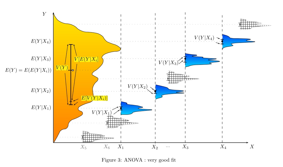
Above we have Young vs old, and short-haired vs long-haired; Pet vs Working breed and less athletic vs more athletic; Weight by breed.
Chi-Squared Tests
Test For Normal Variance
For \(X = X_1, \dots, X_n \sim \N(\mu,\sigma_X^2)\), iid. \[\Null: \sigma = \sigma_0\] \[\frac{(n-1) S_X^2}{\sigma_0^2} \sim \chi^2_{n-1}\] \[\frac{\sqrt{n-1} S_X}{\sigma_0} \sim \chi_{n-1}\]
Goodness of Fit of a Distribution
It is assumed that we have a \(k\) categories with true frequency probabilities \(p_i^*\), \(i=1,\dots,k.\) (multinomial distribution).
The Pearson's cumulative test statistic is given by
\[\chi^2 = \sum_{i=1}^k \frac{(O_i-E_i)^2}{E_i} = n \sum_{i=1}^k \frac{(f_i - p_i)^2}{p_i} \approx \chi^2_{k-1}\] where
\(n\) is the number of observation, \(O_i\) is the number of observations, \(E_i = np_i\) the expected number of observations and \(f_i = O_i/n\) the fraction of observations in group \(i\).
That is \[\Null: E \sim \text{Multinomial}(n,p).\]
For proof of the approximation see here. The counts can be arranged in a frequency table.
For the special case of \(p = (p_1,1-p_1)\) we have \(E_1 \sim \text{Binom}(n,p_1),\) \(E_2 = n-E_1.\) Then \begin{align} \chi_2 &= \frac{(O_1 - np_1)^2}{n p_1} + \frac{(n-O_1 - n(1-p_1))^2}{n (1-p_1)} \\ &= \left( \frac{O_1 - n p_1}{\sqrt{np_1(1-p_1)}}\right)^2 \approx \chi^2_1 \end{align} This test is closely related to the Binomial test.
Test for Statistical Independence
We have two categorical variables \(A,B\) with \(I, J\) levels and \(p_1^*,\dots, p_I^*\), \(q_1^*,\dots, q_J^*\) true probabiliites. \[\chi^2 = \sum_{i=1}^I\sum_{j=1}^J\frac{(O_{ij}-E_{ij})^2}{E_{ij}} = n \sum_{i,j}p_iq_j \left( \frac{O_{ij}/n - p_iq_j}{p_iq_j}\right) \approx \chi^2_{(I-1)(J-1)}\] where \(O_{ij}\) are the sample counts for level \(i\) and \(j\), \(p_i = \sum_j O_{ij} /n \), \(q_j = \sum_i O_{ij} / n\), \(E_{ij} = np_iq_j\) are the expected counts for \(n\) total observations. The counts can be arranged in a contigency table.
Let \(P_{ij}=O_{ij}/n\). If the variables are independent, \[\Null: A \text{ independent from } B,\] we should have have \[P_{ij} \approx p_i q_j \iff O_{ij} \approx E_{ij} \iff \chi^2 \approx 0.\]
If we only have binary categorical variabels and don't have a lot samples we cannot approximate with the chi-squared distribution. We can use FIsher's Exact Test.
Let \(a=P(A=1,B=1),\) \(b=P(A=1,B=0),\) \(c=P(A=0,B=1),\) \(d=P(A=0,B=0).\)
If we have \(n\) samples then for the sample count of \(a\) we have
\[\hat a \sim \text{Hyp}(N=n,M=n(a+c),n=n(a+b)).\]
Tests Based on Rank
Mann-Whiteny U-Test / Wilcoxon Rank Sum Test
For \(X = X_1, \dots, X_n \), iid., \(Y = Y_1, \dots, Y_m \), iid. \[\Null: P(X > Y) = P(Y < X) \text{ or}\] \[\Null: X \text{ and } Y \text{ have same distribution}\] \[U = \sum_{i=1}^n \sum_{j=1}^m S(X_i, Y_j)\] where \begin{align} S(X,Y) = \begin{cases} 1, & \text{ if } Y < X \\ 0.5, & \text{ if } Y = X \\ 0, & \text{ if } Y > X. \\ \end{cases} \end{align}
For small sample size <30 the distribution is tabulated but for large sample size \[\frac{U - \mu_U}{\sigma_U} \approx \N(0,1)\] where \[\mu_U = \frac{nm}{2}, \quad \sigma_U = \sqrt{\frac{mn(n+m+1)}{12}}.\]
Let \(R(X_i)\) denote the rank of \(X_i\) in the combined sample \(X \cup Y.\) Then \[U = \sum_{i=1}^n R(X_i) - \frac{n(n-1)}{2}.\]
If there are observations which share a rank than the standard deviation should be corrected. \[\sigma_U^\text{corr} = \sqrt{\frac{nm}{12}\left((N+1) - \sum_{i=1}^k\frac{t_i^3-t_i}{N(N-1)}\right)}\] where \(N=n+m\) and \(t_i\) is the number of observations sharing rank \(i\) with \(k\) distinct ranks.
Kruskal-Wallis H-test
We have \(k\) independent groups \(Y_i = Y_{ij},\) \(j=1,\dots,n_i\), \(i = 1,\dots,k.\) \[\Null: Y_i \text{ have same distribution}\] \[H = (N-1)\frac{\sum_{i=1}^k n_i (\bar r_i - \bar r)^2}{\sum_{i=1}^k\sum_{j=1}^{n_i}(r_{ij} - \bar r)^2}\] where \(r_{ij}\) denotes the rank of \(Y_{ij}\) in the combined sample, \(\bar r_i\) are the average rank per group \(\bar r = 0.5(N+1)\) is the average rank of all \(N\) observations.
If there are no ties in the ranks then \[H = \frac{12}{N(N-1)} \sum_{i=1}^k n_i (\bar r_i - \bar r)^2\] If there are ties this expression can be corrected by \[H = \left(\frac{12}{N(N-1)} \sum_{i=1}^k n_i (\bar r_i - \bar r)^2 \right) {\huge /} \left(1 - \frac{1}{N^3-N}\sum_{i=1}^g (t_i^3 -t_i)\right)\] where \(t_i\) is again the number of observations sharing rank \(i\) for \(G\) distinct ranks.
For small sample size <30 the distribution is tabulated but for large sample size \[H \approx \chi^2_{k-1}.\]
A significant Kruskal–Wallis test indicates that at least one sample stochastically dominates one other sample.
The Wilcoxon Rank Sum test is the non-parametric equivalent of a two sample unpaired t-test. The Kruskal-Wallis H-test is the non-parametric equivalent of the one-way ANOVA. It extends the Wilcoxon Rank Sum test the same way one-way ANOVA does the two sample unpaired t-test.